Using PyPARRM to filter out stimulation artefacts from data

This example demonstrates how the PARRM algorithm [1] can be used to identify and remove stimulation artefacts from electrophysiological data in the PyPARRM package.

# Author(s):
#   Thomas Samuel Binns | github.com/tsbinns

import numpy as np
from matplotlib import pyplot as plt

from pyparrm import PARRM

Background

When delivering electrical stimulation to bioligical tissues for research or clinical purposes, it is often the case that electrophysiological recordings collected during this time are contaminated by stimulation artefacts. This contamination makes it difficult to analyse the underlying physiological or pathophysiological electrical activity. To this end, the Period-based Artefact Reconstruction and Removal Method (PARRM) was developed, enabling the removal of stimulation arefacts from electrophysiological recordings in a robust and computationally cheap manner [1]. N.B. PARRM assumes that the artefacts are semi-regular, periodic, and linearly combined with the signal of interest.

To demonstrate how PARRM can be used to remove stimulation arfectacts from data, we will start by loading some example data. This is the same example data used in the MATLAB implementation of the method (neuromotion/PARRM), consisting of a single channel with ~100 seconds of data at a sampling frequency of 200 Hz, and containing stimulation artefacts with a frequency of 150 Hz.

data = np.load("example_data.npy")
sampling_freq = 200  # Hz
artefact_freq = 150  # Hz

print(
    f"`data` has shape: ({data.shape[0]} channel, "
    f"{data.shape[1]} timepoints)\n"
    f"`data` duration: {data.shape[1] / sampling_freq :.2f} seconds"
)

`data` has shape: (1 channel, 19130 timepoints)
`data` duration: 95.65 seconds

Finding the period of the stimulation artefacts

Having loaded the example data, we can now find the period of the stimulation artefacts, which we require to remove them from the data. Having imported the PARRM object, we initialise it, providing the data, its sampling frequency, and the stimulation frequency.

After this, we find the period of the artefact using the find_period method. By default, all timepoints of the data will be used for this, and the initial guess of the period will be taken as the sampling frequency divided by the artefact frequency. The settings for finding the period can be specified in the method call, however the default settings should suffice as a starting point for period estimation.

The period is found using a grid search, with the goal of minimising the mean squared error between the data and the best fitting sinusoidal harmonics of the period found with linear regression. The process is described in detail in Dastin et al. (2021) [1], and is also demonstrated in this video from the paper’s authors.

parrm = PARRM(
    data=data,
    sampling_freq=sampling_freq,
    artefact_freq=artefact_freq,
    verbose=False,  # silenced to reduce pqdm output clutter
)
parrm.find_period()

print(f"Estimated artefact period: {parrm.period :.4f}")

Estimated artefact period: 1.3311

Creating the filter and removing the artefacts

Now that we have an estimate of the artefact period, we can design a filter to remove it from the data using the create_filter method. When creating the filter, there are four key parameters:

1. The size of the filter window, specified with the filter_half_width parameter. This should be chosen based on the timescale on which the artefact shape varies. If no such timescale is known, the power spectra of the filtered data can be inspected and the size of the filter window tuned until artefact-related peaks are sufficiently attenuated.

2. The number of samples to omit from the centre of the filter window, specified with the omit_n_samples parameter. This parameter serves to control for overfitting to features of interest in the underlying data. For instance, if there is a physiological signal of interest known to occur on a particular timescale, an appropriate number of samples should be omitted according to this range of time.

3. The direction considered when building the filter, specified with the filter_direction parameter. This can be used to control whether the filter window takes only previous samples, future samples, or both previous and future samples into account, based on their position relative to the centre of the filter window.

4. The period window size, specified with the period_half_width parameter. The size of this window should be based on changes in the waveform of the artefact, which can be estimated by plotting the data on the timescale of the period and identifying the timescale over which features remain fairly constant. This parameter controls which samples are combined on the timescale of the period.

If you are unsure of what parameters are best for your data, you can use the interactive parameter exploration tool offered in PyPARRM (see the explore_filter_params method and the associated example: Exploring the best filter parameters for your data).

Here, we specify that the filter should have a half-width of 2,000 samples, ignoring those 20 samples adjacent to the centre of the filter window, considering samples both before and after the centre of the filter window, and finally using a half-width of 0.01 samples in the period space.

Once the filter has been created, it can be applied using the filter_data method, which returns the artefact-free data. By default, filter_data will filter the data stored in the PARRM object, however other data can be provided should you wish to filter this instead. The filter itself, as well as a copy of the filtered data, can be accessed from the filter and filtered_data attributes, respectively.

parrm.create_filter(
    filter_half_width=2000,
    omit_n_samples=20,
    filter_direction="both",
    period_half_width=0.01,
)
filtered_data = parrm.filter_data()  # other data to filter can be given here

Inspecting the results

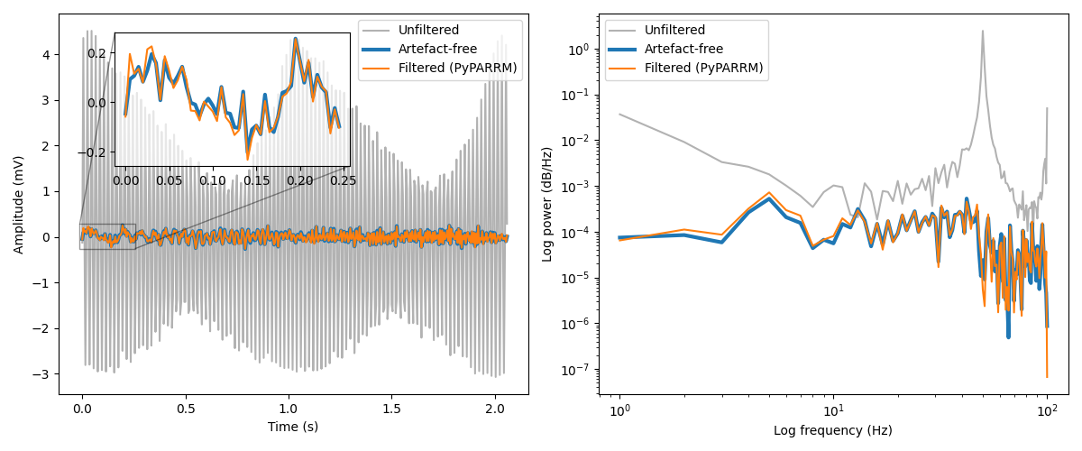
Having filtered the data, we can now compare the results to the original data, as well as the artefact-free form of this simulated data to see how well the method is able to remove the underlying artefacts.

As you can see, the filtered timeseries data closely resembles the true artefact-free data. Furthermore, inspecting the power spectra shows just how well PARRM is able to attentuate the overwhelming power at the 50 Hz subharmonic of the stimulation artefacts, again bringing the results closely in line with those of the true artefact-free data.

# comparison to true artefact-free data
artefact_free = np.load("example_data_artefact_free.npy")
start = 598  # same start time as MATLAB example
end = 1011  # same end time as MATLAB example
times = np.arange(end - start) / sampling_freq

fig, axes = plt.subplots(1, 2, figsize=(12, 5))
inset_axis = axes[0].inset_axes((0.12, 0.6, 0.5, 0.35))

# main timeseries plot
axes[0].plot(
    times, data[0, start:end], color="black", alpha=0.3, label="Unfiltered"
)
axes[0].plot(
    times, artefact_free[0, start:end], linewidth=3, label="Artefact-free"
)
axes[0].plot(times, filtered_data[0, start:end], label="Filtered (PyPARRM)")
axes[0].legend()
axes[0].set_xlabel("Time (s)")
axes[0].set_ylabel("Amplitude (mV)")

# timeseries inset plot
inset_axis.plot(times[:50], artefact_free[0, start : start + 50], linewidth=3)
inset_axis.plot(times[:50], filtered_data[0, start : start + 50])
axes[0].indicate_inset_zoom(inset_axis, edgecolor="black", alpha=0.4)
inset_axis.patch.set_alpha(0.7)

# power spectral density plot
from pyparrm._utils._power import compute_psd

n_freqs = sampling_freq / 2
psd_freqs, psd_raw = compute_psd(
    data[0, start:end], sampling_freq, int(n_freqs * 2)
)
_, psd_filtered = compute_psd(
    filtered_data[0, start:end], sampling_freq, int(n_freqs * 2)
)
_, psd_artefact_free = compute_psd(
    artefact_free[0, start:end], sampling_freq, int(n_freqs * 2)
)

axes[1].loglog(
    psd_freqs, psd_raw, color="black", alpha=0.3, label="Unfiltered"
)
axes[1].loglog(
    psd_freqs, psd_artefact_free, linewidth=3, label="Artefact-free"
)
axes[1].loglog(psd_freqs, psd_filtered, label="Filtered (PyPARRM)")
axes[1].legend()
axes[1].set_xlabel("Log frequency (Hz)")
axes[1].set_ylabel("Log power (dB/Hz)")

fig.tight_layout()
fig.show()

Python vs. MATLAB implementation comparison

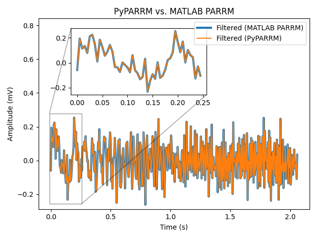
Due to rounding errors, the final filtered data timeseries of PyPARRM and the MATLAB implementation are not perfectly identical (as shown by the failure of numpy.all()), however they are extremely close (as shown by the success of numpy.allclose()). Visual inspection of the plots further demonstrates this similarity. Accordingly, both implementations are suitable for identifying and removing stimulation artefacts from electrophysiological recordings.

# filtered data computed in MATLAB
matlab_filtered = np.load("matlab_filtered.npy")

fig, axis = plt.subplots(1, 1)
inset_axis = axis.inset_axes((0.12, 0.6, 0.5, 0.35))

# main plot
axis.plot(
    times,
    matlab_filtered[0, start:end],
    linewidth=3,
    label="Filtered (MATLAB PARRM)",
)
axis.plot(times, filtered_data[0, start:end], label="Filtered (PyPARRM)")
axis.legend()
axis.set_xlabel("Time (s)")
axis.set_ylabel("Amplitude (mV)")
axis.set_title("PyPARRM vs. MATLAB PARRM")
ylim = axis.get_ylim()
axis.set_ylim(ylim[0], ylim[1] * 3)

# inset plot
inset_axis.plot(
    times[:50], matlab_filtered[0, start : start + 50], linewidth=3
)
inset_axis.plot(times[:50], filtered_data[0, start : start + 50])
axis.indicate_inset_zoom(inset_axis, edgecolor="black", alpha=0.4)

fig.tight_layout()
fig.show()

print(
    "Are the results of the implementations identical? "
    f"{np.all(filtered_data == matlab_filtered)}\n\n"
    "Are the results of the implementations extremely close? "
    f"{np.allclose(filtered_data, matlab_filtered)}"
)

Are the results of the implementations identical? False

Are the results of the implementations extremely close? True

References

[1] (1,2,3)

Evan M. Dastin-van Rijn, Nicole R. Provenza, Jonathan S. Calvert, Anusha B. Allawala, Radu Darie, Sohail Syed, Evan Matteson, Gregory S. Vogt, Michelle Avendano-Ortega, Ana C. Vasquez, Nithya Ramakrishnan, Denise N. Oswalt, Kelly R. Bijanki, Robert Wilt, Philip A. Starr, Sameer A. Sheth, Wayne K. Goodman, Matthew T. Harrison, and David A. Borton. Uncovering biomarkers during therapeutic neuromodulation with PARRM: Period-based Artifact Reconstruction and Removal Method. Cell Reports Methods, 1(2):100010, 2021. doi:https://doi.org/10.1016/j.crmeth.2021.100010.