Exploring the best filter parameters for your data

This example demonstrates how the PyPARRM interactive parameter explorer can be used to find the best filter settings for your data.

# Author(s):
#   Thomas Samuel Binns | github.com/tsbinns

Background

Once you have an estimate of the artefact period, you need to design a filter to remove the artefacts from your data. There are four key filter parameters:

1. The size of the filter window. This should be chosen based on the timescale of which the artefact shape varies.

2. The number of samples to omit from the centre of the filter window. This parameter serves to control for overfitting to features of interest in the underlying data.

3. The direction considered when building the filter. This can be used to control whether the filter window takes only previous samples, future samples, or both previous and future samples into account, based on their position relative to the centre of the filter window.

4. The period window size. The size of this window should be based on changes in the waveform of the artefact. This parameter controls which samples are combined on the timescale of the period.

These parameters are described in detail in Dastin et al. (2021) [1] and the supplementary video from the paper’s authors. Crucially, visualising the effects of these parameters can help greatly for identifying the best settings to use when creating a filter for your data.

Exploring the filter parameters

Once you have an an estimate of the artefact period (see the following example for a detailed explanation of how to do this: Using PyPARRM to filter out stimulation artefacts from data), you can now visualise the effects of the filter parameters to find those that best remove the stimulation artefacts from the data. To do this, we call the explore_filter_params method.

The explorer consists of four plots, and a set of controls:

• The textboxes and buttons in the bottom left of the explorer allow you to manipulate the filter settings. The default settings of the explorer reflect the settings that would be used when computing the filter if you did not specify any inputs. You can change: the period half-width (period_half_width); the filter half-width (filter_half_width); the number of omitted samples (omit_n_samples); and the filter direction (filter_direction). The ranges of possible values that can be entered in the textboxes are shown in brackets.

• The top left plot shows the data samples in the period space according to the current period half-width. Just below this is an overview plot of all the samples in the period space. The red area shows the region currently being viewed in the top left plot. The period space can be moved through using the left and right arrow keys. With these plots, you can find a suitable period half-width, such that the waveform of the artefact remains fairly constant (i.e. a straight line could easily be drawn through the plotted samples in period space). Furthermore, as you change the filter half-width, these plots will reflect the change in the number of available samples.

• Most importantly, the two plots on the right-hand side show the unfiltered and filtered data according to the current filter settings in the time domain (top plot) and in the frequency domain (bottom plot). Both plots are updated in real-time according to changes in the filter settings. The power spectral density is particularly useful for identifying which filters reduce the signal’s power at the artefact frequency (as well as at the harmonics and sub-harmonics). In some cases, the filter settings may not produce a valid filter, in which case a warning on the time domain plot will be printed.

If computational cost is a concern, a limited time range of the data and its resolution can be specified, as well as the frequency range and resolution of the power spectral density. If multiple channels are present in your data, these can be navigated between using the up and down arrow keys. Finally, the title of the explorer gives you an overview of the current filter settings, as well as which channel’s data is currently being viewed.

The method can be called as parrm.explore_filter_params(). The image below shows the different aspects of the parameter explorer window.

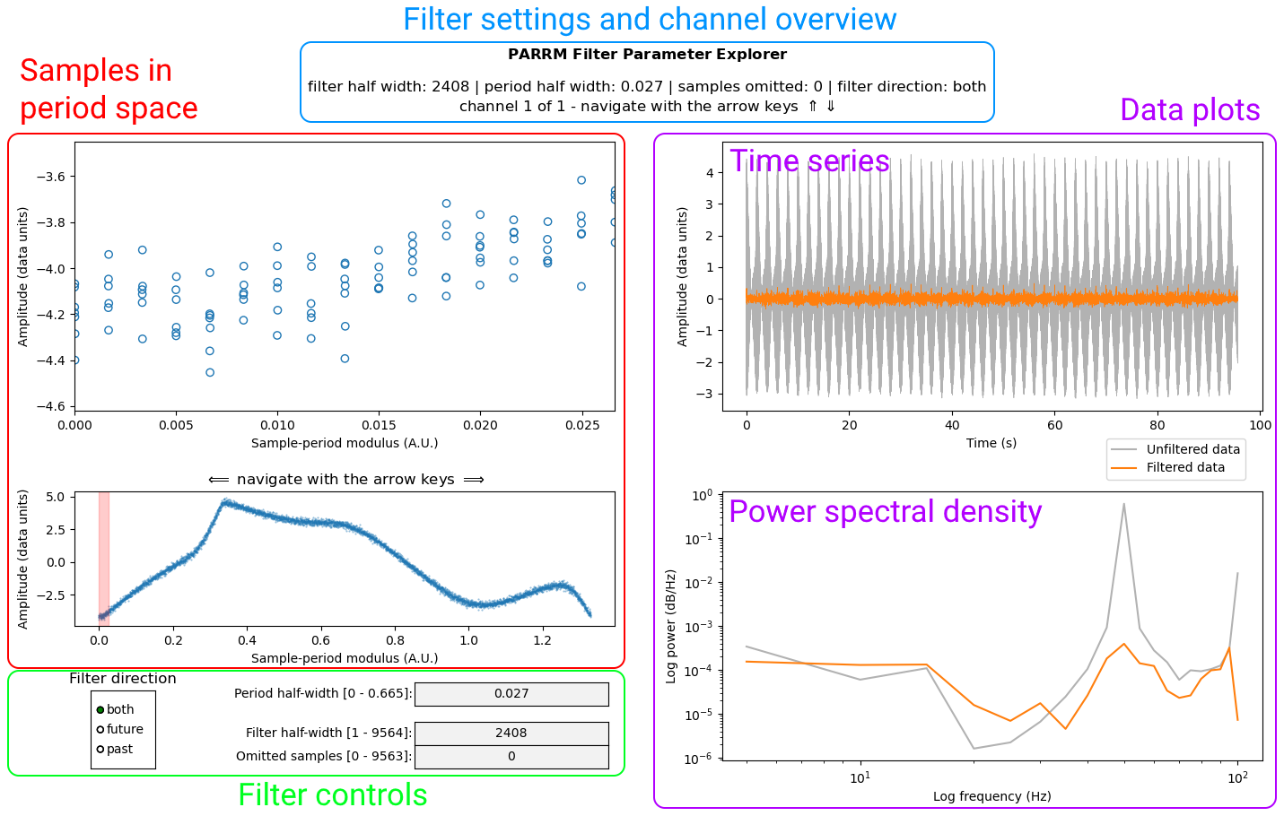
An overview of the parameter explorer window features