Real data example: stimulation artefacts in human ECoG data

This example demonstrates the utility of PARRM [1] on a genuine recording of human brain activity from local field potentials (LFPs) at the site of deep brain stimulation in the subthalamic nucleus, and from electrocorticography (ECoG) at the cortex.

# Author(s):
#   Timon Merk          | github.com/timonmerk
#   Thomas Samuel Binns | github.com/tsbinns

import numpy as np
from matplotlib import pyplot as plt

from pyparrm import PARRM

Background

Deep brain stimulation (DBS) is an established treatment for several disorders such as Parkinson’s disease, epilepsy, and dystonia. In subjects undergoing DBS, brain activity can also be recorded. Unfortunately, the quality of signals recorded at not only the site of stimulation, but often from distal regions too, can be detrimentally affected by stimulation-related artefacts.

In this example from a Parkinson’s disease patient undergoing DBS of the subthalamic nucleus - a common target for stimulation - we show how PARRM can be used to remove stimulation artefacts from both LFP recordings of the subthalamic nucleus and ECoG recordings of cortical activity.

We start by loading some ECoG and LFP data collected during rest, each consisting of an individual channel spanning 60 seconds, with a sampling frequency of 1,000 Hz. DBS was delivered at a frequency of 130 Hz.

data_ecog_lfp = np.load("ecog_lfp_data.npy")

sampling_freq = 1000  # Hz
artefact_freq = 130  # Hz

Finding the artefact period and filtering the data

When handling data from multiple sites, the decision must be made whether to estimate the period of the stimulation artefacts for this data separately, or together. Assuming that the stimulation artefacts have a similar effect on the subthalamic and cortical signals, we can take advantage of the more efficient approach of estimating the period for all data simultaneously. However, if differences in the period between recording sites are of a particular concern, we can also estimate the periods separately. Below, we estimate the periods on: the ECoG and LFP data together; the ECoG data alone; and the LFP data alone. In this case, the estimate of the periods are identical to 5 decimal places. Nevertheless, if you can afford the increased computational cost, you may see improved performance for estimating the period independently for recordings from different sites.

Having estimated the period, we proceed to create a filter and apply it to the data. The following examples give a detailed explanation of the process for finding the artefact period and filtering the data, as well as for finding the optimal filter parameters for your data: Using PyPARRM to filter out stimulation artefacts from data; Exploring the best filter parameters for your data.

parrm = PARRM(
    data=data_ecog_lfp,
    sampling_freq=sampling_freq,
    artefact_freq=artefact_freq,
    verbose=False,
)
parrm_ecog = PARRM(
    data=data_ecog_lfp[[0]],
    sampling_freq=sampling_freq,
    artefact_freq=artefact_freq,
    verbose=False,
)
parrm_lfp = PARRM(
    data=data_ecog_lfp[[1]],
    sampling_freq=sampling_freq,
    artefact_freq=artefact_freq,
    verbose=False,
)

parrm.find_period()
parrm_ecog.find_period()
parrm_lfp.find_period()

parrm_ecog.create_filter(period_half_width=0.02, filter_half_width=5000)
parrm_lfp.create_filter(period_half_width=0.01, filter_half_width=3000)

filtered_ecog = parrm_ecog.filter_data()
filtered_lfp = parrm_lfp.filter_data()

print(
    f"Artefact period (ECoG & LFP): {parrm.period :.7f}\n"
    f"Artefact period (only ECoG):  {parrm_ecog.period :.7f}\n"
    f"Artefact period (only LFP):   {parrm_lfp.period :.7f}"
)

Artefact period (ECoG & LFP): 7.7424022
Artefact period (only ECoG):  7.7424027
Artefact period (only LFP):   7.7424017

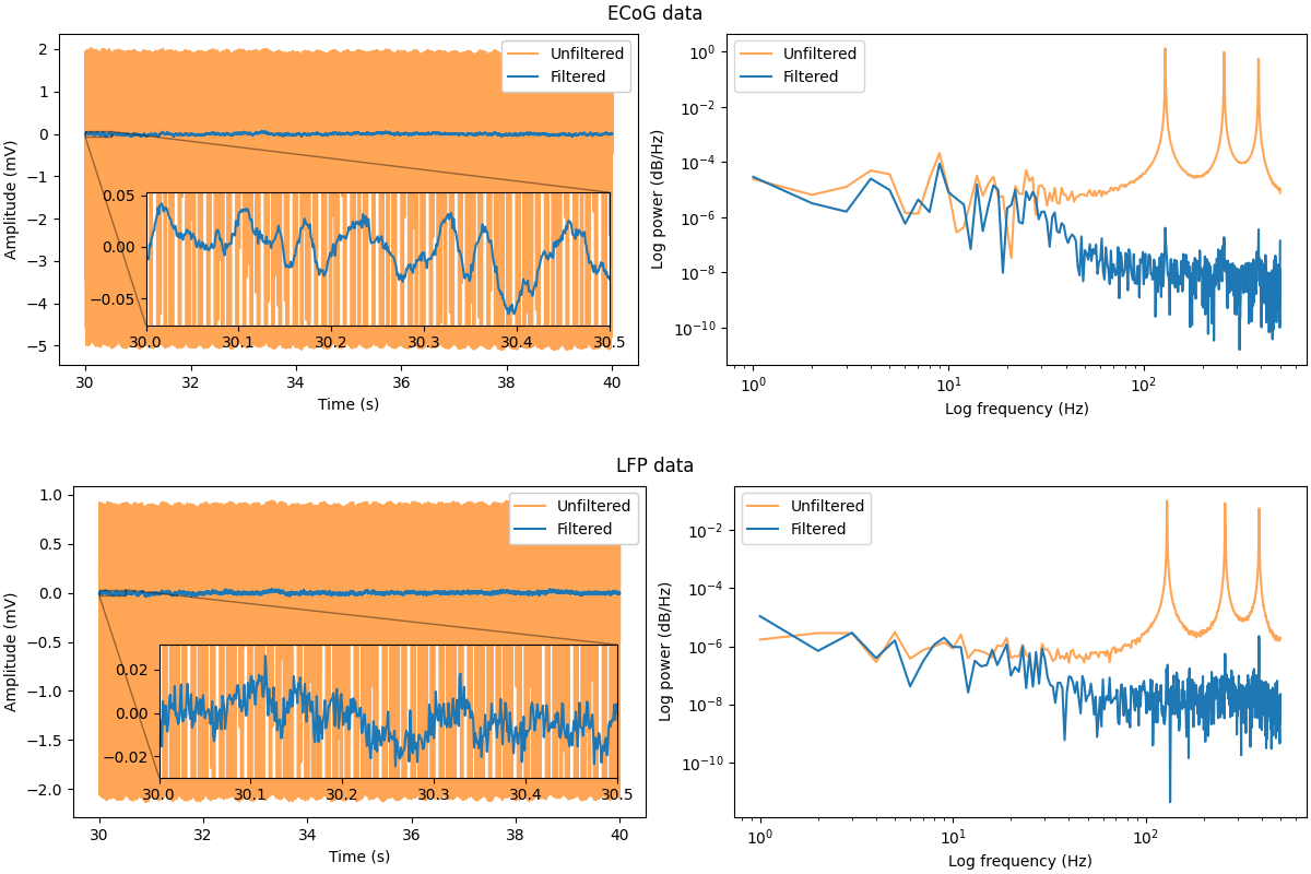
Inspecting the results

Having filtered the data, we can now compare the results to the original, artefact-contaminated signals. The plots below show the entire 60 second timeseries of the data, as well as the power spectral densities across this period.

For both the ECoG and LFP data, the reduction in power at the 130 Hz stimulation frequency and its harmonics (260 Hz and 390 Hz) is readily apparent. Whilst some spikes in power at these frequencies remain, the activity is much less broadband, and as such the information in the neighbouring frequencies is less compromised. Finally, it can be seen that PARRM performs well for both the ECoG data from the cortex - located distally from the site of stimulation - as well as for the LFP data - collected at the site of DBS.

Altogether, it is clear that PARRM is a powerful tool for removing periodic stimulation artefacts from electrophysiological data in a computationally-efficient manner.

# times to plot
times = np.arange(30, 40.0001, 1 / sampling_freq)
start_idx = 30 * sampling_freq
end_idx = 40 * sampling_freq
inset_times = np.arange(30, 30.5001, 1 / sampling_freq)
inset_start_idx = 30 * sampling_freq
inset_end_idx = int(30.5 * sampling_freq)

from pyparrm._utils._power import compute_psd

n_freqs = sampling_freq / 2
psd_freqs, psd_unfiltered = compute_psd(
    data_ecog_lfp, sampling_freq, int(n_freqs * 2)
)
_, psd_filtered_ecog = compute_psd(
    filtered_ecog, sampling_freq, int(n_freqs * 2)
)
_, psd_filtered_lfp = compute_psd(
    filtered_lfp, sampling_freq, int(n_freqs * 2)
)

fig = plt.figure(figsize=(12, 8), layout="constrained")
subfigs = fig.subfigures(2, 1, hspace=0.07)
data_idx = 0
for data_name, filtered_data, filtered_psd in zip(
    ["ECoG", "LFP"],
    np.concatenate((filtered_ecog, filtered_lfp)),
    np.concatenate((psd_filtered_ecog, psd_filtered_lfp)),
):
    axes = subfigs[data_idx].subplots(1, 2)
    inset_axis_time = axes[0].inset_axes((0.15, 0.12, 0.8, 0.4))
    subfigs[data_idx].suptitle(f"{data_name} data")

    # timeseries
    axes[0].plot(
        times,
        data_ecog_lfp[data_idx, start_idx : end_idx + 1],
        color="#ff7f0e",
        alpha=0.7,
        label="Unfiltered",
    )
    axes[0].plot(
        times,
        filtered_data[start_idx : end_idx + 1],
        color="#1f77b4",
        label="Filtered",
    )
    inset_axis_time.plot(
        inset_times,
        data_ecog_lfp[data_idx, inset_start_idx : inset_end_idx + 1],
        color="#ff7f0e",
        alpha=0.7,
    )
    inset_axis_time.plot(
        inset_times,
        filtered_data[inset_start_idx : inset_end_idx + 1],
        color="#1f77b4",
    )
    inset_axis_time.set_xlim(30, 30.5)
    inset_data = filtered_data[inset_start_idx : inset_end_idx + 1]
    inset_ylim_pad = (np.max(inset_data) - np.min(inset_data)) * 0.1
    inset_ylim = np.array(
        (
            np.min(inset_data) - inset_ylim_pad,
            np.max(inset_data) + inset_ylim_pad,
        )
    )
    inset_axis_time.set_ylim(inset_ylim)
    axes[0].indicate_inset_zoom(inset_axis_time, edgecolor="black", alpha=0.4)
    axes[0].legend(loc="upper right", framealpha=1)
    axes[0].set_xlabel("Time (s)")
    axes[0].set_ylabel("Amplitude (mV)")

    # power spectral density
    axes[1].loglog(
        psd_freqs,
        psd_unfiltered[data_idx],
        color="#ff7f0e",
        alpha=0.7,
        label="Unfiltered",
    )
    axes[1].loglog(psd_freqs, filtered_psd, color="#1f77b4", label="Filtered")
    axes[1].legend(loc="upper left")
    axes[1].set_xlabel("Log frequency (Hz)")
    axes[1].set_ylabel("Log power (dB/Hz)")

    data_idx += 1

fig.show()